
Excel explained: part one
Excel… what is it? The Exhibition Centre in London? Nope. When you do something well, better than others? Well yes, it could be. In this case, though, we’re talking about the Microsoft software used to create spreadsheets – and the format all our Flourish tools are built in.

If you’re not sure how to use Excel, don’t panic. That’s exactly what this free resource is here to help you with. And once you’ve mastered these basics and can use your tools confidently, you can boost your spreadsheet skills even more with Excel, Explained… a bit more.
Google Sheets is a free alternative to Excel, but unfortunately the functionality of the Flourish tools disappears when you convert between the two. If you don’t have Excel, we can build you a custom tool in Sheets instead. Just get in touch!
Let’s start with the basics – what is a spreadsheet?
A spreadsheet is an electronic document where data is arranged in cells. The cells are arranged in rows and columns, and data which is put in these cells can be manipulated and used in calculations.
A brief introduction – meet Excel…
In Excel, every file is called a ‘workbook’. You can have several pages within each workbook, each called ‘worksheets’. You will find tabs to access your different worksheets in the bottom left-hand corner of your workbook.

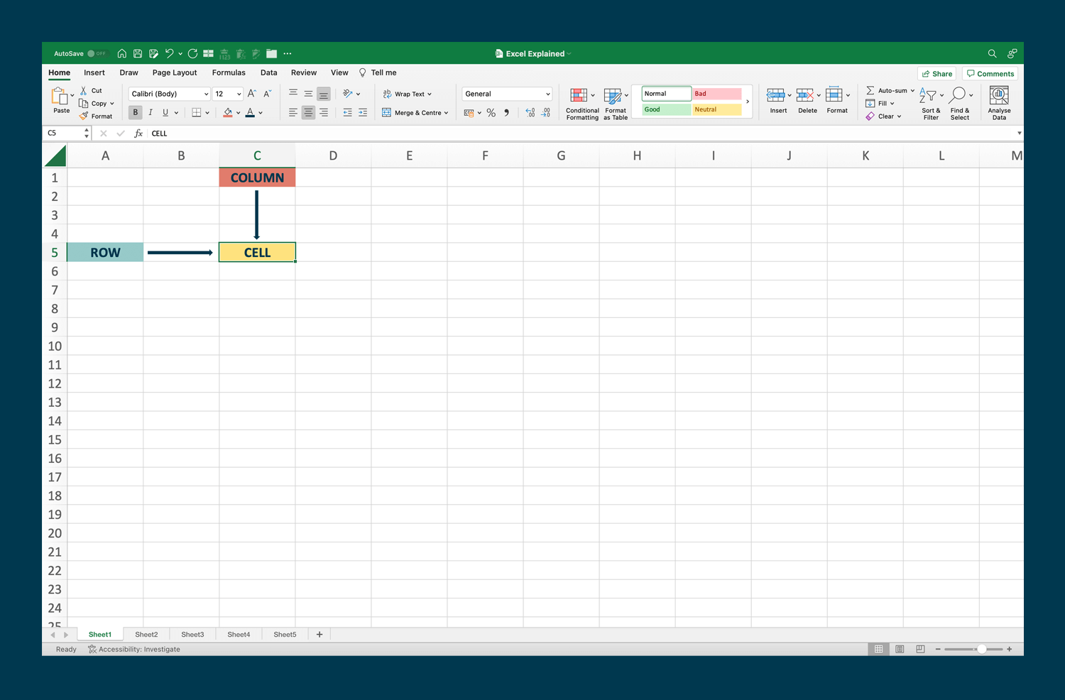
Across the top of your worksheet are ‘columns’, which run vertically. These are lettered from A to XFD; that's an amazing 16,384 columns. Don’t worry, we won’t use them all!
Down the side of your worksheet are ‘rows’, which run horizontally. These are numbered from 1 to 1,048,576. Wow.
The point where a column and a row cross is called a ‘cell’. Each cell is referenced by the column letter and row number, i.e. C5.
How to open your Flourish tool in Excel
When you buy a Flourish tool, you’ll find it in your ‘Downloads’ folder.
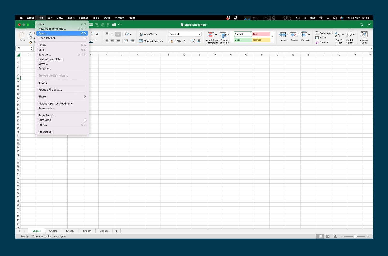
In the menu bar at the top of the page, select 'File’ and then ‘Open’ from the drop-down menu. A list of your folders will appear.
Select the ‘Downloads’ folder by double-clicking on it with your cursor, and then find your Flourish tool in the list of files. Click on it with your cursor to select it and then click ‘Open’ in the bottom right-hand corner.

How to save a workbook in Excel
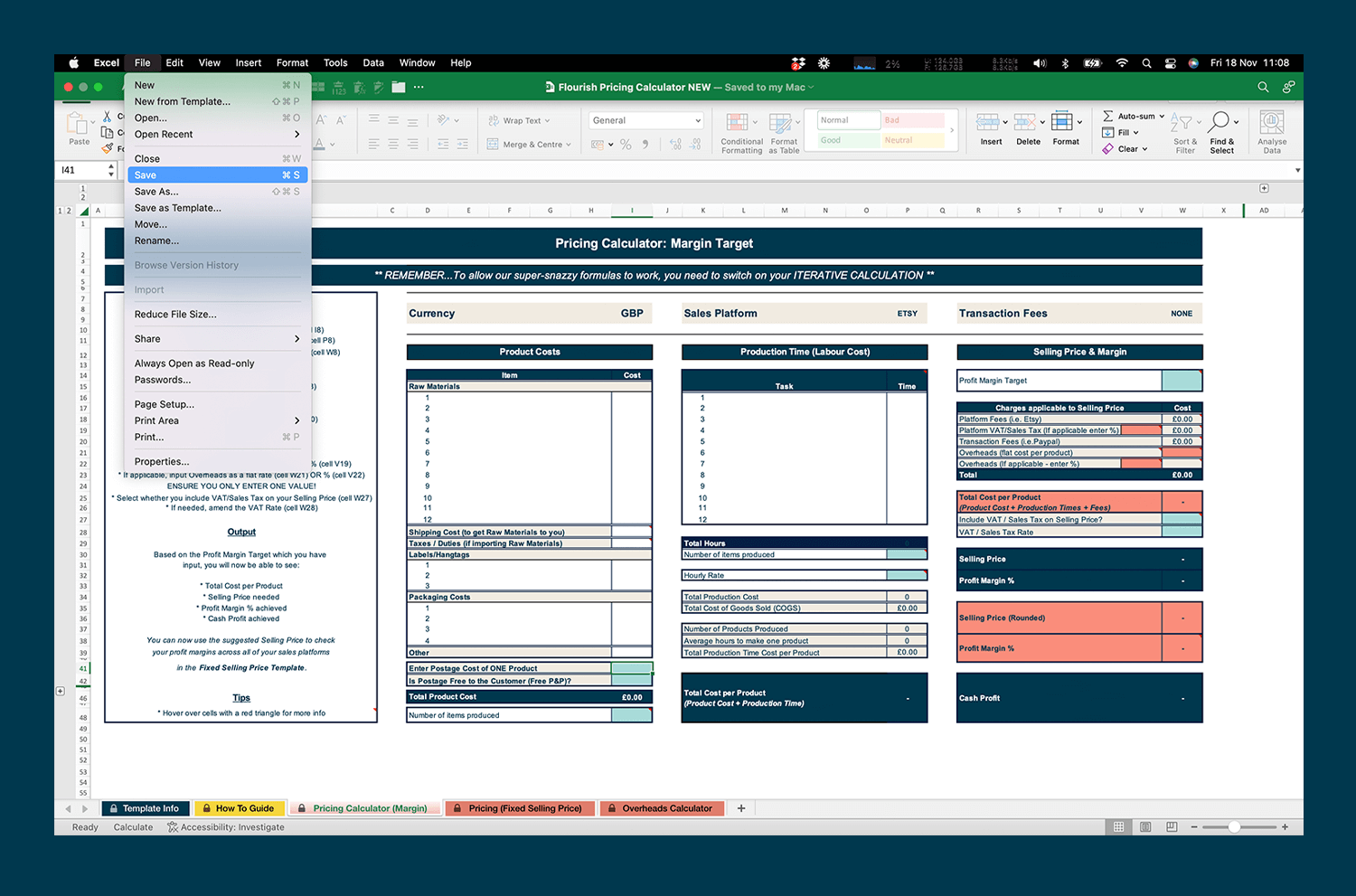
Once you’ve opened your Flourish tool, you’ll want to save it in a folder. With the workbook open, select ‘File’ from the menu bar at the top. Then select ‘Save’ from the drop-down menu that appears.
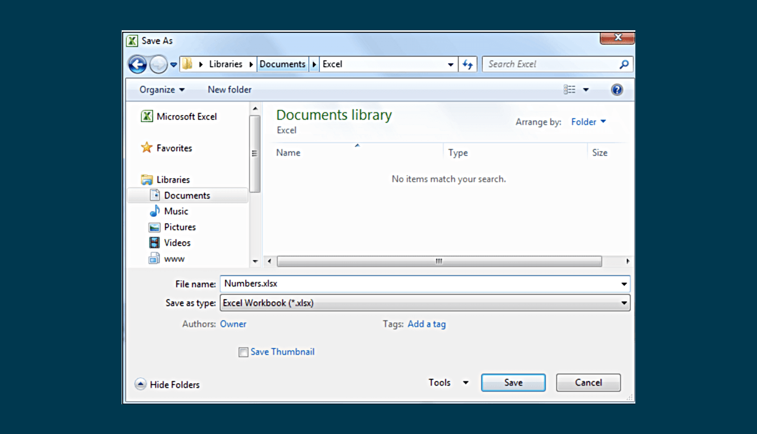
If the file hasn’t been saved previously, a ‘dialog’ box will appear, in this case called ‘Save As’. In the box, there will be a suggested name, based on the file either being a new workbook (i.e. Book7) or a download (i.e. Flourish Pricing Calculator).
You can stick with this name or choose your own name. If you choose to re-name your workbook, type the new name in the ‘Save As’ box, deleting the suggested one.
Where it will be saved will be shown in the aptly named ‘Where’ box. If you want to change that location, click on the blue arrows and select your preferred folder.
Once you’re happy with the name and where the file will be saved, hit the ‘Save’ button in the bottom right-hand corner of the dialog box.
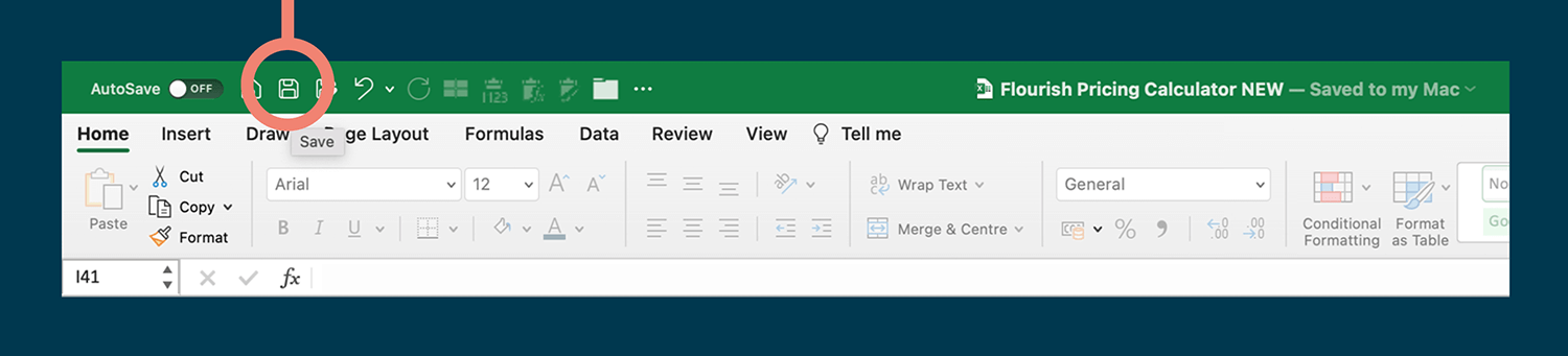
Once a sheet has been saved, use the floppy disk icon (shown below – so very vintage!), to quickly save any future changes.
If you’re saving on a mac:
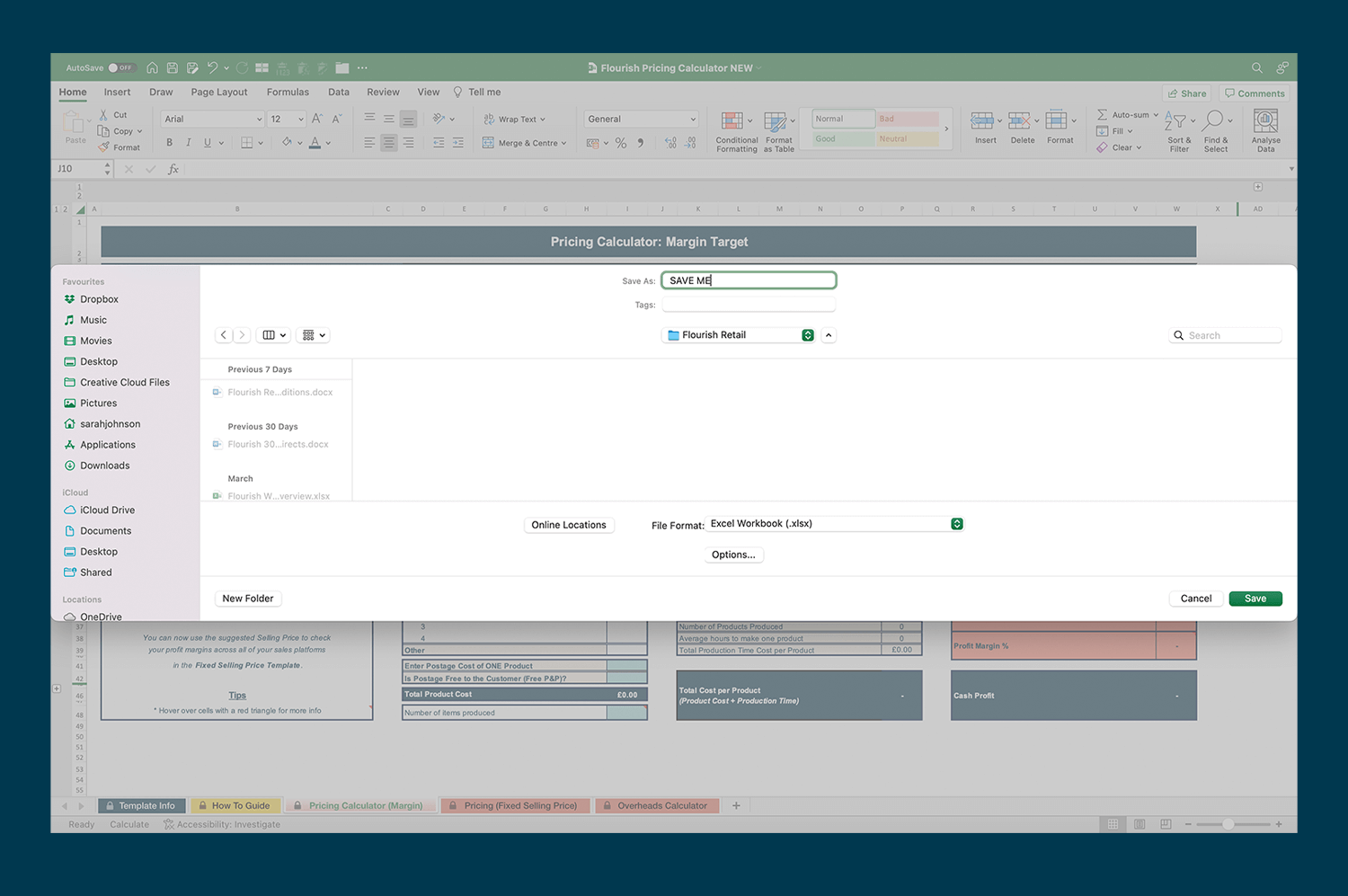
If you haven’t saved a file before on the Mac, a dialog box will appear. The ‘Save As’ box will be showing a suggested name, based on it either being a new workbook (e.g. Book1) or a download (e.g. Pricing Calculator). If you want to re-name your workbook, type the new name in the ‘Save As’ box.
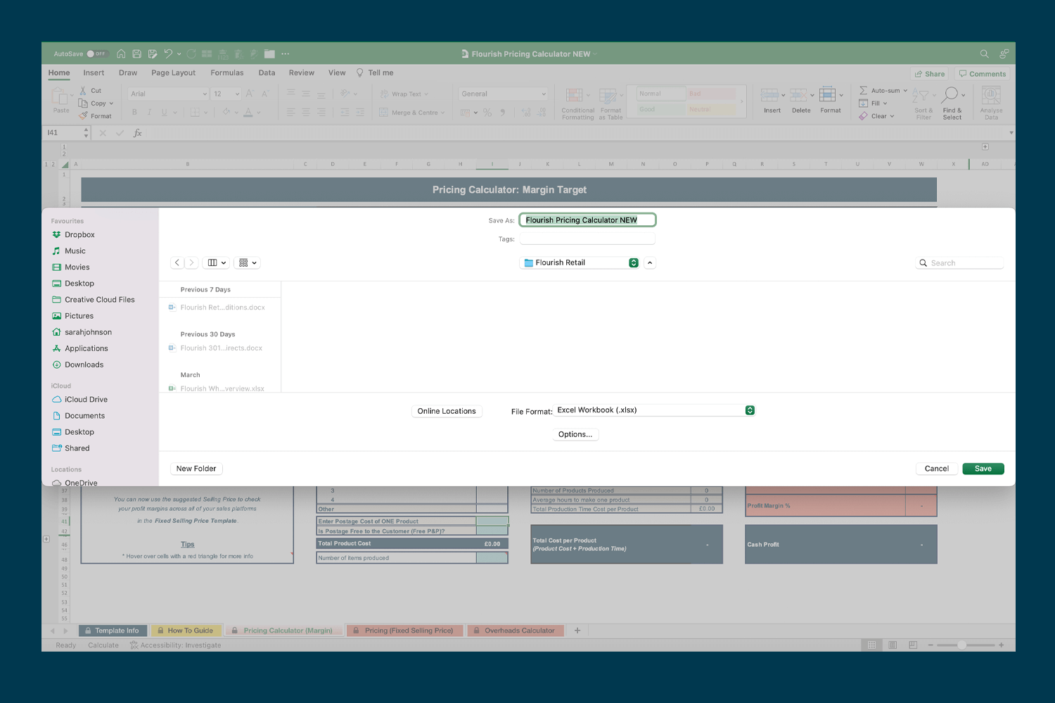
The aptly named Where box then lets you choose the folder you want to save it in. Click on the green arrows.
Once you’re happy with the name and the folder, click the ‘Save’ button in the bottom right-hand corner.
How to resolve ‘circular references’ messages
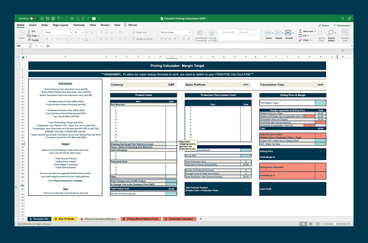
Some of our super-snazzy formulas work off a circular reference (basically, when a formula refers back to its cell and gets a bit confused). In order for them to work beautifully, you’ll need to switch on your ‘iterative calculation’. Sounds complicated but fear not, it’s easy!
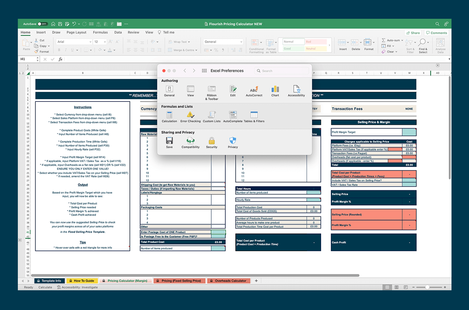
In the top left-hand corner, hover over Excel & click on ‘Preferences’.
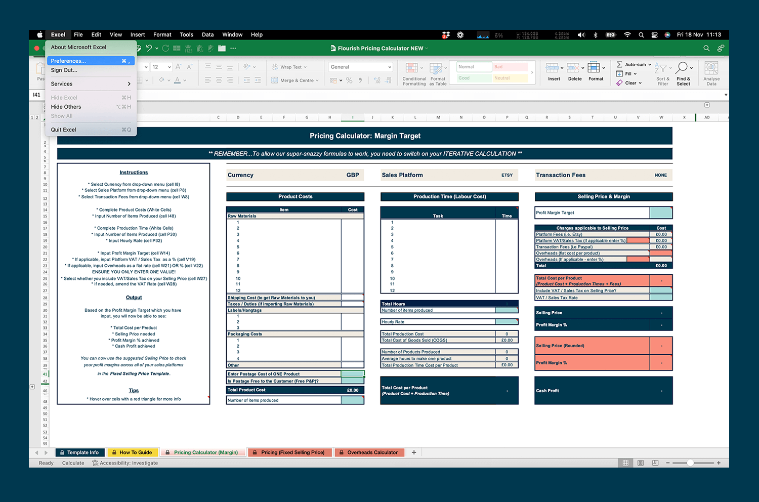
Under ‘Formulas & Lists’, select ‘Calculation’.
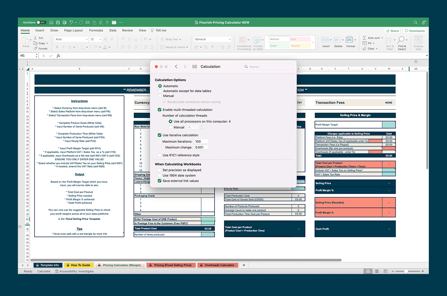
Select ‘Use Iterative Calculation’ (a tick should appear) and you’ll be good to go.
How to enter data into a cell
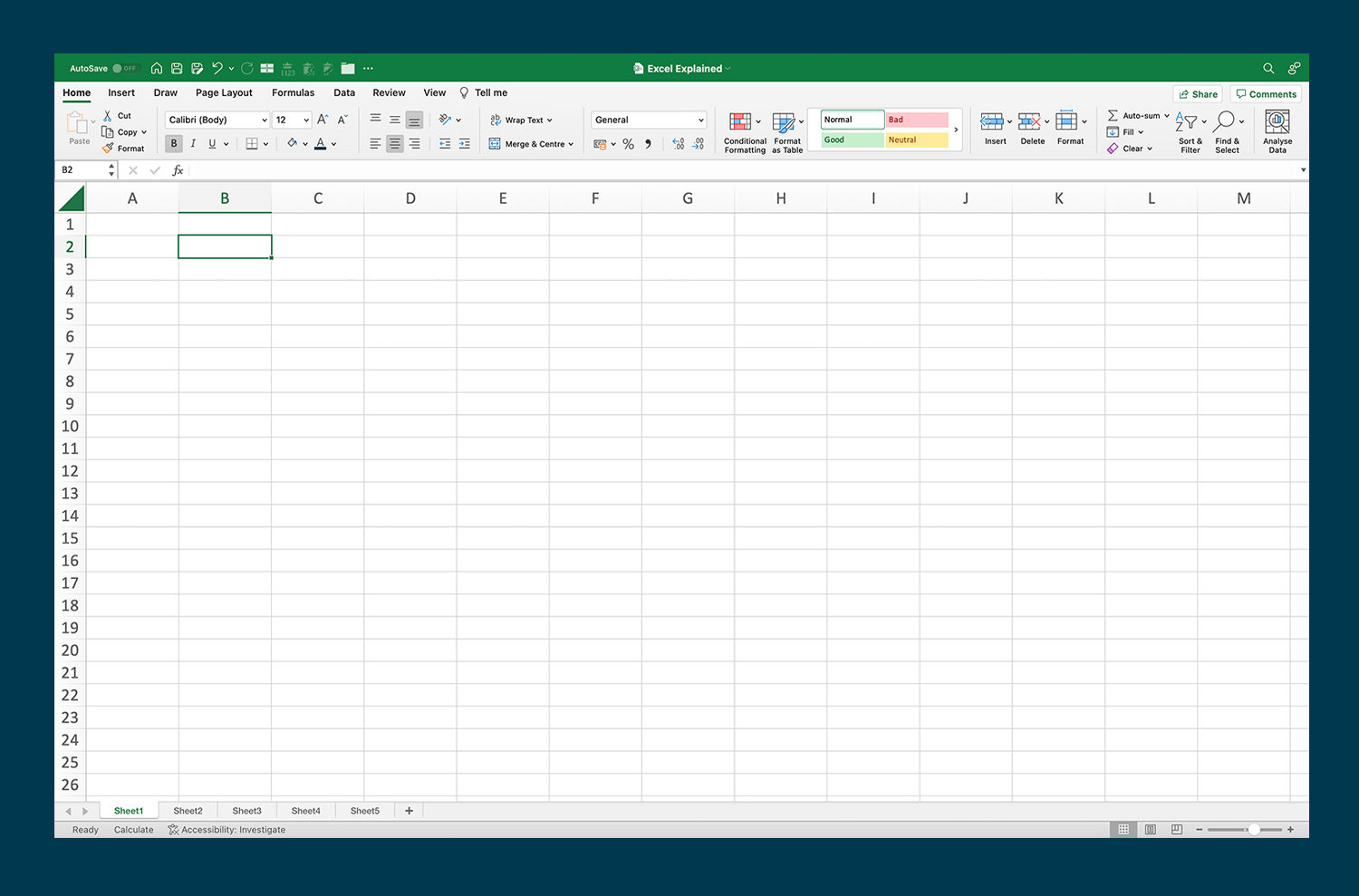
First, select your cell by pointing your cursor at it and clicking. In the example below, we’re selecting cell B2.
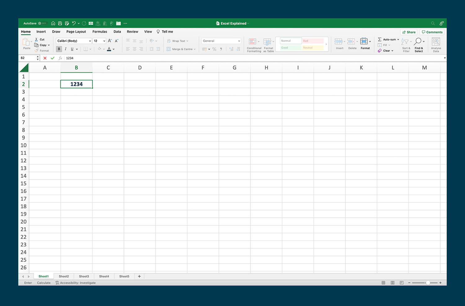
Once the cell has been selected, type in your text or numbers. You might notice that the information you type also appears in the Formula Bar above the column headers. Once you’ve typed what you want to, click out of the cell and into another one.
How to add a row in Excel
In some of our trackers, you may want to add additional rows. You can do this by selecting the last cell of the table by pointing your cursor there and clicking on it.
Next, press ‘Tab’ on your keyboard. The new row will appear with all of the relevant formulas and formatting.
How to move between worksheets in Excel
You’ll find each worksheet named on the tabs at the bottom of your workbook. You can move between them by clicking the worksheet tab you want to display.

Viewing ‘comments’ in Excel
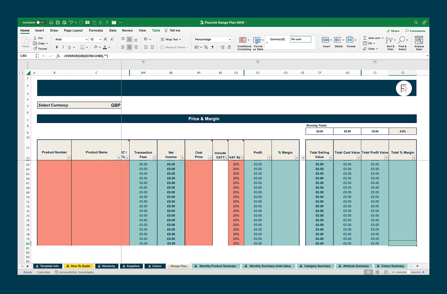
When you use your Flourish tools, you may notice small red triangles in the corners of some cells. These are comments, and they’re usually an explanation, calculation or helpful tip for you to use. You can see the comment by hovering your cursor over the red triangle.
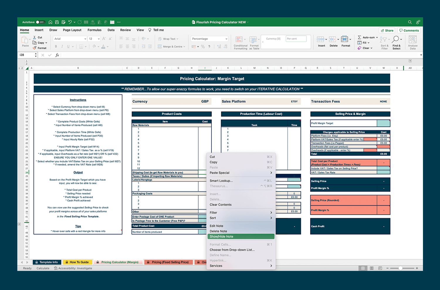
If that’s not working for some reason, right-click on the cell and select ‘Show Comment’ from the drop-down menu. You can hide it again by right-clicking on the cell and selecting ‘Hide Comment’.
Congratulations! You’ve mastered the basics of Excel
Give yourself a pat on the back and celebrate with a cuppa. You deserve it. After all, you now know all the basic skills you need to use your Flourish tools with confidence.
There’s always more, though. If you want to learn some extra tips and tricks to help you get even more from those tools, check out Excel, Explained… a bit more.