
Excel explained: part two
If you’ve already mastered all the basics in Excel explained: part one, this free resource brings you a few more tips, tricks, hints and help to get a bit more from your Flourish tools. Happy spreadsheet-ing!

How to open a workbook you’ve already saved to your computer
In the menu bar at the top of the page, select ‘File’ and then ‘Open’ from the drop-down menu. A list of your folders will appear.
Double-click on the folder where you’ve saved the file and then select the file by clicking on it with your cursor. Then click ‘Open’ in the bottom right-hand corner.
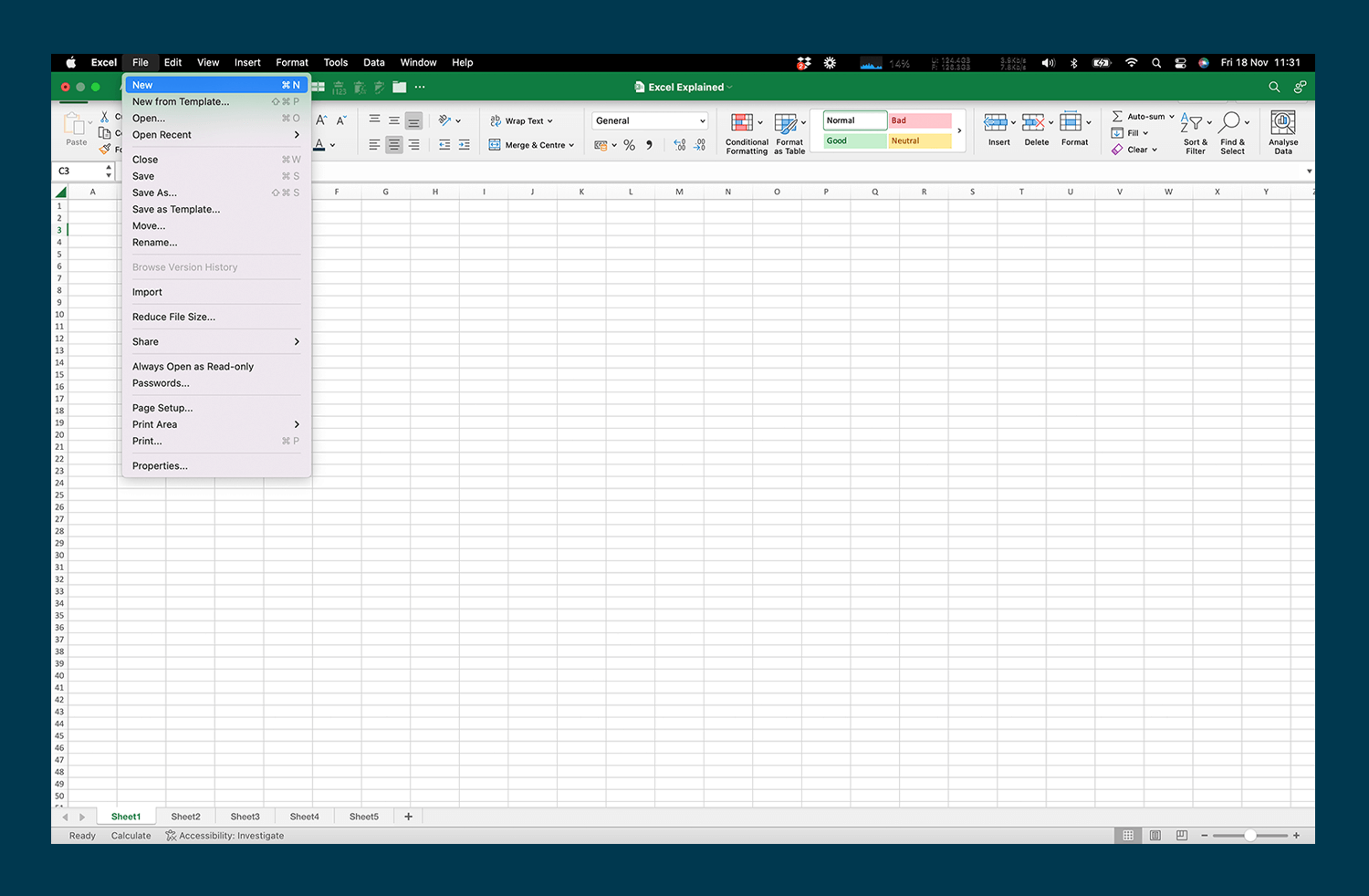
How to create a brand new workbook in Excel
At the top of your screen you’ll see the menu bar. Use this to select ‘File’. Then select ‘New’. Your new workbook will appear.
How to re-order your worksheets
If you want to, you can re-order the worksheets within your workbook. To do this, hold your cursor down on the tab that you would like to move until a small black arrowhead appears.

Still holding the cursor down on the tab, drag it across to its new position and then release the cursor. You’ll see the other worksheets adjust around the one that’s been moved.

The joy of the Excel formula!
A formula is the way you tell your worksheet to ‘do’ something to the data you’ve entered. Often the ‘doing’ is a mathematical calculation.
In Excel you can write your own formulas, or use pre-defined ones, called Functions.
You’ll recognise a formula because it always starts with an equal sign (=) and is typed into the Formula Bar just above your column headers*. All of the Flourish tools have been created with formulas which will save you time and give you the perfect answer.

*Some of the formulas in your Flourish tools will be hidden or locked so you don’t accidentally change, or get distracted by them. Some of them are pretty long.
Filtering your data
Filters are really useful, because they let you specify criteria within your worksheet. Any rows which meet the criteria you’ve picked will show, and any which don't are hidden. That’s really handy if you have a lot of data and need to find something or if you want to just look at a specific type of product!
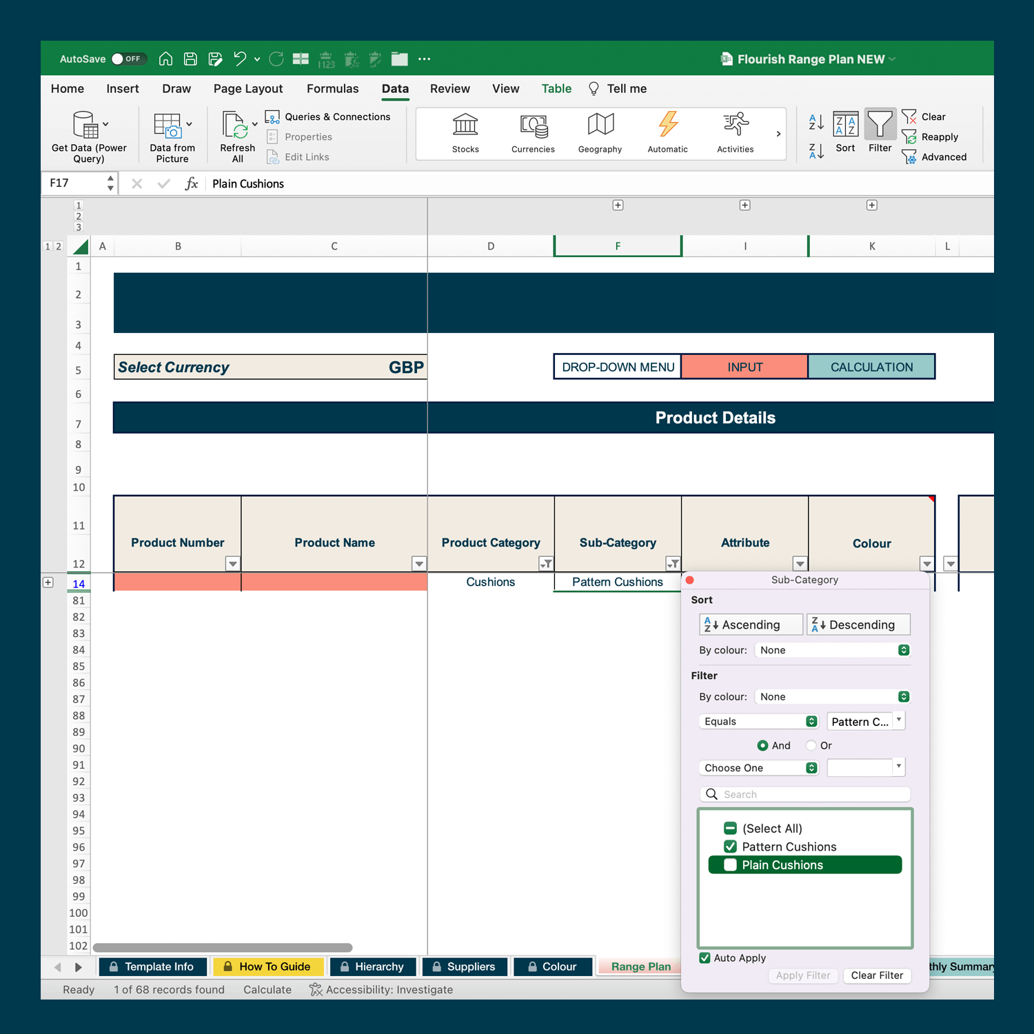
To add filters, select the ‘Data’ tab at the top of the screen and click the ‘Filter’ icon in the toolbar. You’ll see small arrows appear next to each column heading in your tool.

Choose which column you would like to filter on (e.g. Product Category), and click on the small arrow in that column. A dialog box will appear with all of the options from the data in that column (e.g. cushions, lampshades, rugs, blanks).

Click the ‘Select All’ box to unselect all the options. Then select your criteria by clicking the relevant box (e.g. cushions). A green tick will appear, and your data will filter as shown below.

You can filter by more than one criteria – just select more than one option (e.g. cushions AND rugs)! Rows containing those options will be displayed, while the other, unchecked options will remain hidden.

To show all of your data again, click the ‘Select All’ box. And voila! You'll be able to see all of your data again.

Using filters on more than one column:
You can also filter by more than one column. Each new column you filter will be based on the choices you have already made in previous columns (e.g. cushions > plain cushions), so the data will keep reducing.
Removing filters:
To remove your filters completely, go back to the ‘Data’ tab and click the ‘Filter’ icon again. All of your filters will be removed, and the small arrow icons will disappear. You can switch them back on again whenever you want.

Sorting your data
There are some clever sorting elves embedded in our Flourish tools, which means that your analysis will always show you sales from highest to lowest. But if you'd like to do your own sort, here's how:
First, select the ‘Data’ tab and click the ‘Sort’ icon in the toolbar.

A dialog box will appear.

Select the column you want to use to sort your data by clicking on the drop-down menu, using the up and down arrows.

You can choose what to ‘Sort On’ (e.g. Values, Cell Colours etc.), and you can also select the ‘Order’ you want to sort your data in (e.g. Descending (A-Z), Ascending (Z-A), or a custom option). Once you’ve selected the options you want, click ‘OK.’ Your data will be highlighted and sorted to your selection.

To undo the sorting, click the ‘Undo’ button above the ‘Formulas’ tab.

Grouped rows and columns
In some of your tools, you might notice that some rows or columns are hidden. In these cases you’ll see a gap in the sequence of numbers (rows) or letters (columns), and a small ‘+’ sign above or to the left of the sheet.

You can unhide those rows or columns by clicking on those ‘+’ icons (i.e. D, F and I). Alternatively, you can unhide them ALL by clicking on the small ‘2’ icon on the left-hand side.

You’ll now see the ‘-’ icon and a line above the column(s) or next to the row(s) included in the grouping.
If you want to hide them again, just click on the relevant ‘-’ icons, or hide them all by clicking the small '1' icon on the left-hand side.
Note: Some columns contain data for formulas, so they’re just hidden to keep things tidy. If you accidentally unhide them, you’ll spot HIDE above them. Others are hidden to save space on the worksheet, and you will have instructions for these with your tool.
How to print a worksheet in Excel
To print your worksheet, you’ll first need to check the page layout. If you’re working from a Flourish tool, this will generally be set for you already.
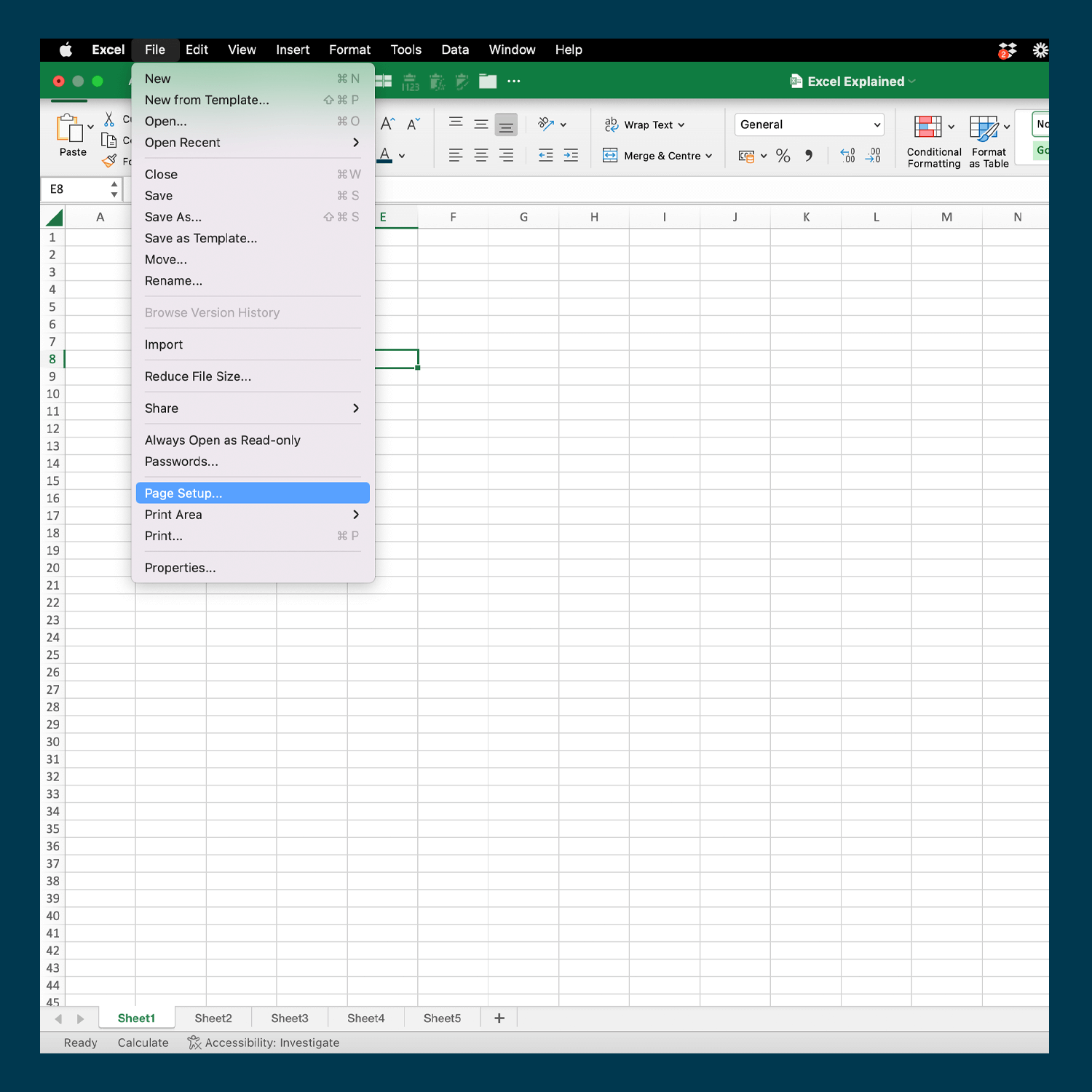
If you’re not working on a Flourish tool, you can do this by selecting ‘File’ from the menu bar at the top, then clicking on ‘Page Setup’.
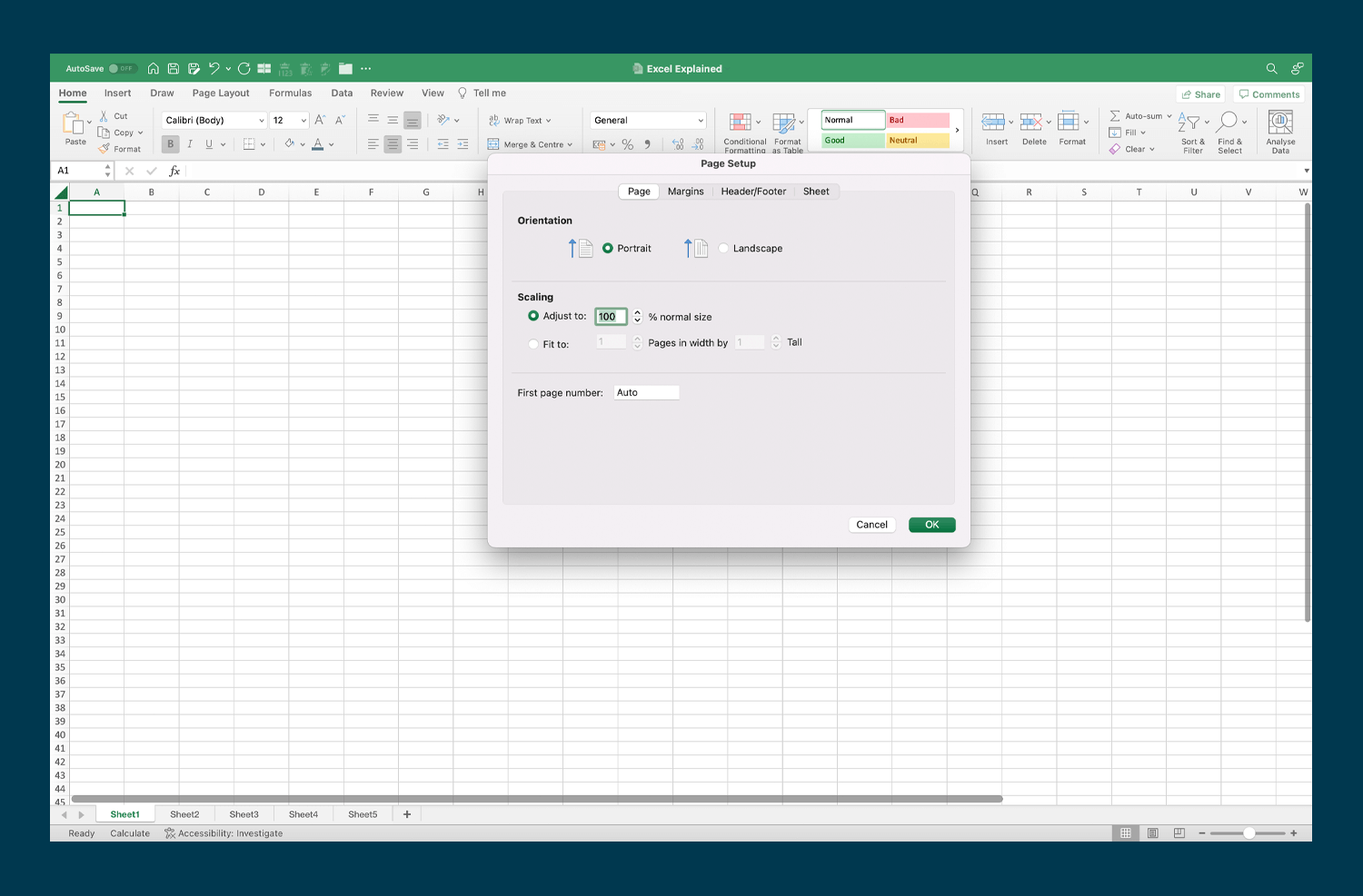
A dialog box will appear with the following options:
Orientation: This is the way around the paper will print, and will already be set for your tool. In the example below, Portrait is selected; shown with a green and white circle.
To change it, click the white circle next to the other option (i.e. Landscape).Scaling: This lets you fit your worksheet to a set number of pages. Your Flourish tools will usually be designed to fit on one page, but sometimes they 'grow', as more lines get added. For these, you may need to increase the number of pages 'tall', so that it is legible.
Happy with your selection? Click OK.
Now go back to the menu bar at the top, select ‘File’ and then ‘Print’ from the drop-down list. Your page will be sent to your printer!

Using Excel to analyse data
In Excel you can create graphs and charts which help you to identify trends and make the best decisions for your business. You can learn more about analysis in our free resource about Tracking and Analysing Your Sales!

You’re good to go, Excel pro!
Now that you understand a bit more about using our Flourish tools, you might find yourself itching to add more options to the tools. That’s fine! We can add that extra functionality you need to make the tools work perfectly for your business. Just get in touch!